Exoplanet Weather Goes 3D with JWST's Map of WASP-18b

Breaking through the flat-sky ceiling

On October 28, 2025, astronomers published the first full three dimensional map of a planet’s atmosphere beyond the Solar System. The target was WASP-18b, an ultra hot Jupiter about 400 light years away. Researchers used a technique called 3D eclipse mapping to turn a single, exquisite observation from NASA’s James Webb Space Telescope into a weather map with latitude, longitude, and altitude. The result reads like a CAT scan of an alien world: a blistering dayside hotspot encircled by a cooler ring near the limbs, and signatures that water vapor is torn apart in the hottest region. You can read the study’s technical backbone in the Nature Astronomy study on WASP-18b.

What makes this moment a step change is not only the image in our heads of a planetary hotspot, but the ability to resolve structure vertically. Until now, most exoplanet “maps” were flat snapshots that averaged over layers of air like a long exposure. With altitude in play, we can separate surface weather from stratospheric chemistry, and rewiring that distinction reshapes how we search for life.

How 3D eclipse mapping works

Imagine watching a city skyline at sunset. As buildings pass into shadow, the fading light traces their shapes. Eclipse mapping is similar, but the roles are reversed: when a transiting planet slips behind its star, the planet’s dayside goes dark from our point of view. The exact shape of that fading and reappearing light carries a fingerprint of how brightness is distributed across the planet’s face. For a very different kind of eclipse experiment, see Proba-3’s artificial eclipses.

Two pieces make the map three dimensional:

Longitude: As the planet moves behind the star, different east–west slices disappear first. The fine structure in the light curve tells you which longitudes are bright or dim.
Latitude: During the brief ingress and egress, the star’s limb scans north–south zones. That brief interval contains the latitudinal information.
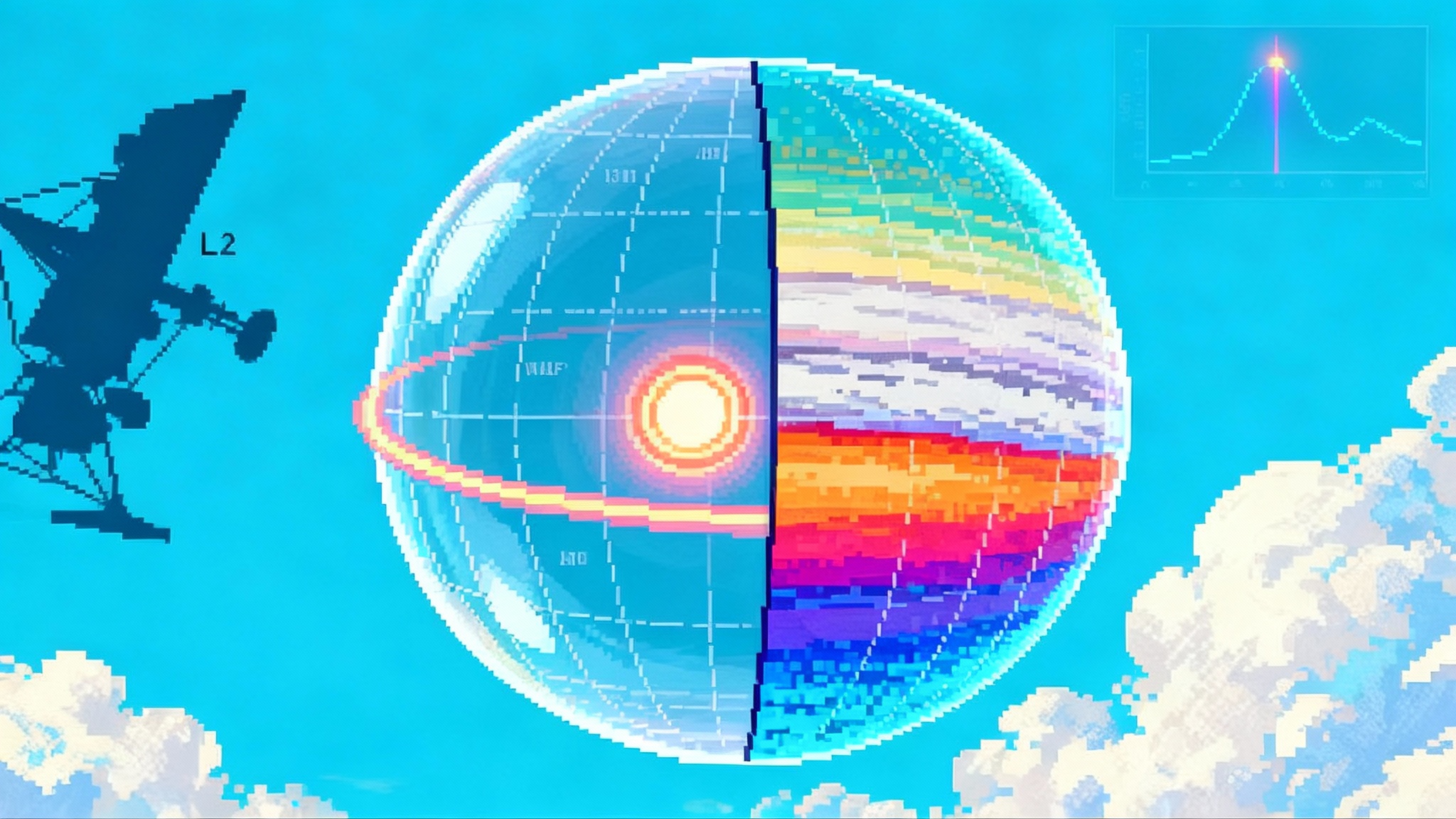
Altitude: Webb’s instruments split the light into many colors. Each color probes a different pressure level, because gases absorb and emit at specific wavelengths and depths. Stack brightness maps at several colors and you get altitude layers, much like geological strata in a canyon wall.

For WASP-18b, the team used Webb’s Near Infrared Imager and Slitless Spectrograph to take a spectroscopic movie across the secondary eclipse. They inverted that movie into a set of temperature maps. By comparing maps at wavelengths where water absorbs to maps where it does not, they pinpointed layers where water is present and layers where extreme heat likely breaks water apart into hydrogen and oxygen atoms. That difference is the altitude dimension doing real work.

What the WASP-18b map actually shows

WASP-18b is tidally locked, which means the same hemisphere always faces its star. The map reveals:

A compact, nearly circular hotspot centered close to the substellar point. Models predicted eastward offsets driven by fierce jet streams, but this hotspot sits more squarely under the star. That implies drag on the winds, possibly from magnetic effects or strong radiative cooling that kills the jets before they can move heat sideways.
A cooler ring near the dayside limbs. This ring forms where air begins to slide toward the night, a region known as the terminator. Temperatures plunge by hundreds of degrees between the hotspot and this ring.
Lower water abundance in the hotspot than the hemispheric average. The simplest explanation is thermal dissociation. At several thousand degrees, water molecules cannot survive; they break into constituent atoms, which recombine in cooler zones as air circulates.

This last point sounds subtle, but it matters. If you took a single spectrum averaged over the hemisphere, you would see a muted water signal and might infer that the whole atmosphere is dry. The map shows the opposite: the planet has water, but it is chemically stratified by heat. Without the altitude dimension, that nuance is invisible.

Why altitude is the step change

On Earth, the difference between cloud decks and the stratosphere is everything. Thunderstorms live in the troposphere. Ozone chemistry lives higher up. The same logic extends to exoplanets. If you cannot separate vertical layers, you mix weather and climate into a single smear.

Altitude clarity unlocks three upgrades:

Causality instead of correlation. A spectrum alone can tell you that water features are weak. A 3D map can tell you why. In WASP-18b, weak features line up with the hottest layers, where dissociation is expected, and grow stronger where air cools toward the limbs. That cause-and-effect breaks degeneracies in retrieval models.
Dynamics with teeth. Wind patterns are not just east–west conveyor belts. The relative sizes of the hotspot and the cooler ring constrain how quickly air rises, moves, and sinks. The team found weaker longitudinal temperature gradients than some general circulation models predicted, pointing to processes like hydrogen dissociation cooling and recombination heating that blunt the day–night contrast. Comparisons to volcanic heat transport, such as Juno’s record Io eruption, show how energy sources shape flows.
Chemistry in 3D. Many claimed biosignatures are products of disequilibrium, meaning they should not persist unless something replenishes them. To prove disequilibrium you must know where gases are made, destroyed, or stored across altitude. That requires vertical structure.

From hot Jupiters to the next wave of targets

Hot Jupiters like WASP-18b are ideal training grounds. They are big, bright, and short period, which gives high signal and frequent eclipses. But the method is not limited to these giants. Here is how 3D mapping scales.

Sub Neptunes. Puffier worlds like GJ 1214 b and K2 18 b have large eclipse depths and well placed infrared features. Multi color eclipse maps can distinguish high altitude hazes from deep humidity and can test whether methane and carbon dioxide reside in separate layers. Even a two layer vertical separation helps resolve the current debate over whether these planets host mini ice giant atmospheres or water rich envelopes.
Lava worlds. Ultra hot rocky planets such as 55 Cancri e and LHS 3844 b present tiny signals but extreme contrasts. A coarse 3D map would reveal whether heat escapes through a bare rock surface or a thin atmosphere shuttling energy to the night. That is a sharp test of atmospheric survival on close in terrestrial planets.
Benchmark Jupiters around bright stars. A handful of nearby gas giants produce the cleanest ingress and egress signatures. These will populate a reference set where latitude–longitude–altitude maps can be compared directly against next generation climate models that include magnetic drag, molecular dissociation, and cloud microphysics.

In each case, the strategy is the same: build layered maps at a few carefully chosen wavelengths, then connect those layers with a physics based retrieval that enforces energy balance and chemistry.

What 2026 to 2030 looks like in practice

A realistic roadmap, grounded in current schedules:

2026 to 2028, JWST follow ups. Webb can repeat the WASP-18b experiment on a half dozen ultra hot Jupiters and several warm Neptunes. The first pass uses Near Infrared Imager and Slitless Spectrograph and Near Infrared Camera grisms for the altitude layers where water and carbon dioxide absorb. A second pass with Mid Infrared Instrument reaches cloud forming pressures. The goal is a small atlas of 3D maps that anchor models across temperature and gravity regimes.
2027 to 2029, Roman Coronagraph. The Nancy Grace Roman Space Telescope is expected to launch no later than May 2027. Its coronagraph is a technology demonstration aimed at direct imaging in reflected light, not transits. That still matters for mapping. In reflected light, phase curves and color changes across an orbit can reveal cloud belts and patchy surfaces on nearby Jupiters, with sensitivity to different altitudes than thermal emission. Roman will help validate techniques that combine reflected light maps with thermal maps to link cloud tops to deeper heat transport.
2029 to 2033, Ariel survey era. The European Space Agency’s Atmospheric Remote sensing Infra Exoplanet Large survey mission is planned to launch in 2029 to study roughly one thousand transiting worlds. Ariel’s uniform instrument setup and repeat visits will turn 3D mapping from boutique to routine. Think of Ariel as the census taker that fills the gaps Webb cannot reach. See the agency’s plan in the ESA mission overview. The year will be busy across planetary science, from OSIRIS-APEX to shadow Apophis to Ariel’s first wide surveys.
2029 to 2030 and beyond, Extremely Large Telescope spectroscopy. The European Southern Observatory’s Extremely Large Telescope expects first test observations in March 2029 and first science in late 2030. Its giant mirror and high resolution spectrographs will resolve individual spectral lines that sharpen wind speeds and pressure levels. When you measure line widths and shifts across ingress and egress, you get a dynamical layer cake: where winds blow, how hard, and how that changes with height.

This sequence is not sequential in a hard sense. It is a cross calibration campaign. Webb pins the thermal layers. Ariel scales the sample. Roman demonstrates reflected light mapping on nearby giants. The Extremely Large Telescope adds crisp velocity profiles with altitude. Together, they produce climate atlases with the vertical resolution needed to test models.

What 3D maps change for biosignature strategies

Claims of life will hinge on ruling out false positives. Three dimensional context helps in four specific ways:

Vertical consistency checks. If you claim methane and oxygen on the same planet, you must show they can coexist without destroying each other. A 3D map lets you ask whether methane hides in a lower layer under an inversion while oxygen sits higher, perhaps supplied by photolysis. That does not prove biology, but it keeps the chemistry honest.
Cloud bias control. Clouds mute or mimic features depending on altitude. Without vertical information you can mistake a cloudy layer for low abundance. Layered maps let you adjust for clouds explicitly by fitting their pressure level and optical depth.
Heat engine tests. Many biosignature gases are destroyed by high temperatures. If a map shows those gases only at the terminator or nightside, that pattern supports survival rather than production. If a gas remains uniform with altitude and longitude despite expected destruction, you have a stronger disequilibrium claim.
Mission design feedback. The community must decide which wavelengths future observatories prioritize. 3D maps show exactly which bands separate layers best for key molecules. That feeds into filter choices and spectrograph ranges for missions like the proposed Habitable Worlds Observatory.

A concrete playbook for the next five years

To avoid hand waving, here are specific actions, with why and how:

Build a reference sample. Select 8 to 12 transiting planets across three bins: ultra hot Jupiters, warm Neptunes, and one or two rocky candidates. For each, obtain two spectroscopic eclipses with Webb at complementary wavelength ranges. This provides redundancy against systematics and spans the altitude range where water, carbon monoxide, carbon dioxide, and silicates dominate.
Standardize the inversion. Adopt a shared pipeline for eclipse mapping with clear tests against overfitting. Require cross validation against a uniform disk model and publish information content metrics. This keeps latitude estimates honest and makes maps comparable across targets.
Couple maps to general circulation models. Do not stop at retrievals. Feed the 3D temperature and composition fields back into climate models that include magnetic drag, dissociation and recombination, and cloud microphysics. Publish forward modeled maps so differences between model and data can be traced to specific physics, not to plotting choices.
Use Roman to test reflected plus thermal synthesis. For two or three bright nearby Jupiters that are not transiting, combine Roman phase resolved reflected light maps with ground based thermal phase curves. The aim is to prove that mixed light sources can still yield consistent vertical structure when tied to a physics based model.
Prepare Ariel target tiers now. Define a small set of Tier 1 objects where Ariel repeats eclipses in multiple channels to recover basic vertical gradients, and a larger Tier 2 set for statistical trends without full maps. This ensures the survey balances depth and breadth from day one.
Plan Extremely Large Telescope follow up on the same targets. High resolution spectroscopy during ingress and egress can measure wind shear with height through line shifts. Schedule those around Ariel and Webb to harvest maximum cross calibration.

Why this is more than a milestone headline

There have been elegant maps before, beginning with two dimensional brightness maps using the Spitzer Space Telescope. The Webb result puts altitude on the map and confirms a theory long sketched in models: on the hottest exoplanets, the chemistry itself is part of the heat engine. Water breaks in the hotspot. Hydrogen atoms carry energy. Recombination releases that energy as air moves into cooler zones. That cycle changes the winds and the emission we see.

From a distance, a spectrum is a single chord. With 3D eclipse mapping, we are hearing the harmony. The next few years will tell us whether that harmony carries to smaller and cooler worlds, where biology might one day be plausible. The way to get there is not mysterious. It is a set of repeatable observations, transparent inversions, and instruments aimed at the exact wavelengths that separate layers.

The bottom line

A three dimensional map of WASP-18b shows that exoplanet weather is no longer a flat picture. Altitude structure is now observable, not inferred. That single shift lets us test dynamics, chemistry, and cloud physics together. With Webb, Ariel, Roman, and the Extremely Large Telescope, the field is poised to turn 3D mapping into a standard diagnostic. That will sharpen our search strategies, refine our mission designs, and make the eventual interpretation of biosignatures far more robust. The sky did not get flatter as we looked farther. It got deeper, and we finally learned how to see it.